How it works

Architecture

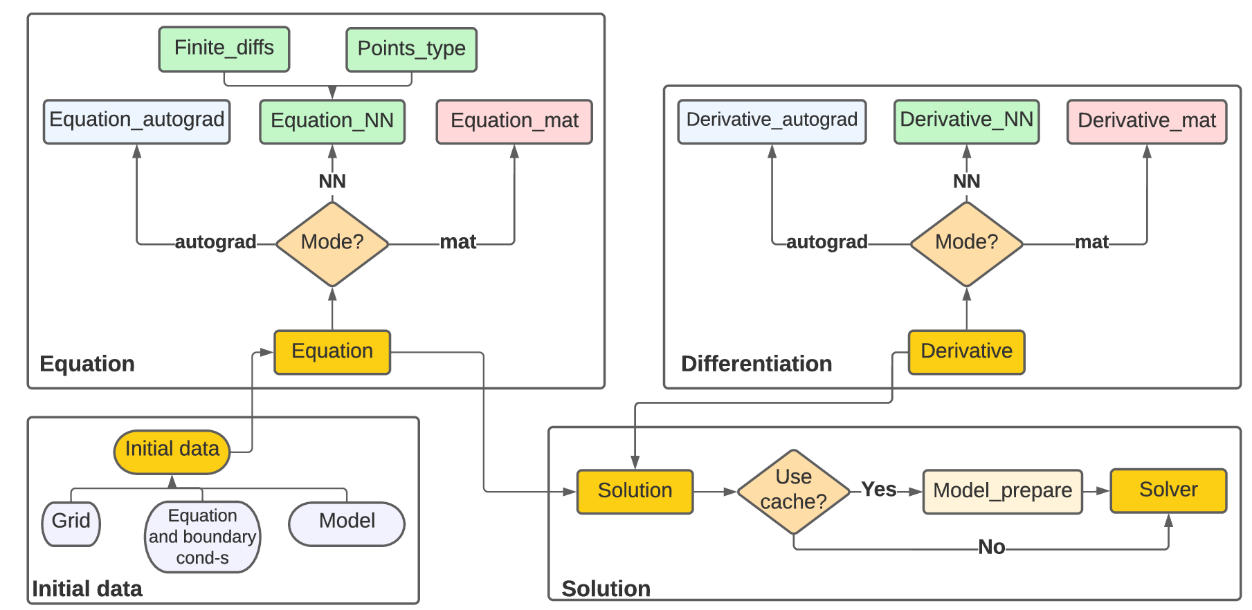
The architecture itself can be represented as in the figure below:

The solver is implemented so that it can be extended with new methods for solving differential equations without global changes in the architecture.

To define a new differential equation solution method, it is necessary to define a new solution method Equation and the mechanism for determining the derivative Derivative.

In TEDEouS, we do not stick to the neural networks - the proposed approach may be extended to an arbitrary parametrized model.

So, let’s move to the each part of architecture.

Equation

The equation module allows to set an O/PDE, boundary and initial conditions, calculation domain.

Moreover, it is possible to choose different approaches to solve an equation. Solver supports methods based on a matrix (linear model without activation layers) and neural network optimizations as well as a method based on pytorch automatic differentiation algorithm.

Grid

The grid parameter represents a domain where we want to calculate a differential equation. The only significant restriction is that only a single-connected domain may be considered. We do not assume that geometry has a particular shape - rectangular, circular or any other analytical domain. To preserve generality domain is represented by the number of points.

Equation

We collect all required parameters to equation interface. Interface includes several parameters such as: coefficient, operator, power and optional parameter variable (it must be specified if the equation depends on 𝑛 variables, i.e. in case of system solution).

Boundary and initial conditions

In the classical solvers, we work with canonical types such as prescribed values (Dirichlet type boundary conditions, it may be a function of boundary) of field or normal differential values (Neumann type boundary conditions) for the entire boundary. Initial conditions are also prescribed values or function at 𝑡 = 0.

Solution

Differenatation